How to Use Freez and Unfreez in Excel

You have lots of data and working on it, you want the first row or the first column of your sheet should be watchable even if you are working on the last cell of your data.

This type of the difficulties is faced by everyone who is working with lots of data.

The solution is to freeze the column or row, where your parameters existed. You can also unfreeze the column and row when your work finished.

"Freeze Panes option is helpful When you are dealing with lots of data"

Step 1:  To select the Rows that you want to Freeze

 

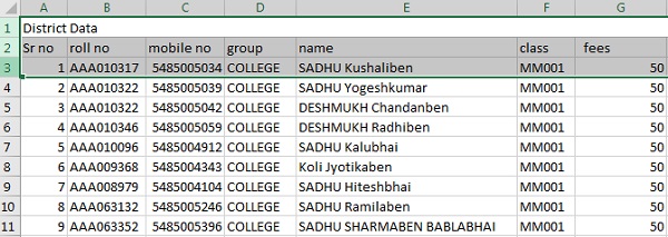
Here we want to freeze the first two columns so we have to select the first three rows of the sheet, in which the first two rows will be freeze.

Step 2: Go to the view option and press Freeze Panes and Select Freeze Panes

After Selecting the first three rows in which we want to Freeze first two rows, click on the View button on the top side of the sheet and search Freeze panes option. Click on freeze panes.

Step 3: The first two rows have Freeze 

Now scroll down the sheet you can see the first two rows are freeze and the rows below are scrolling.

To Unfreeze

Step 4: Now select the Freeze Rows and click on Unfreeze Panes.

It is a reverse process of freeze panes. You have to select the rows you have freeze and click on the view button and then click on Freeze Panes and select Unfreeze Panes. It will unfreeze the first two rows that we have freeze.

Note: 

Here you can Freeze Panes Horizontally and Vertically.

If you want to freeze column and row in the middle of the sheet you can do it by selecting the single row.

Freeze pane is also called a lock.

How would you like this content to write us in the comment box!

If you face any difficulty in the content feel free to ask!

Thank You.